Cube Sort

Cube Sort is a sorting algorithm that uses a binary search cube data structure to store elements before reinserting them back into the array.
How Cube Sort works
The binary search cube is a data structure that works like an n-dimensional array where each axis has indices that are sorted by their index. For example consider this array of the numbers 0-9:
[0, 1, 2, 3, 4, 5, 6, 7, 8, 9]
This can be represented in a 2-dimensional array like this:
[0, 1, 2][3, 4, 5][6, 7, 8, 9]
Then if we want to search for an item, we first do a binary search on the first item of each row and then within that row. So if we want to find 5 within the array we follow these steps:
3is the middle point so we start from comparing5to it.5is greater so we compare it to the midpoint of the upper half,6.5is lower than6, so now it’s narrowed down to the 2nd sub-array.- Now that we know it’s in the 2nd array, we find the middle point:
4. 5is greater than the4, so we know it’s to the right.- We look at the midpoint of the right side of the sub-array and there it is, a
5!
This process is used in Cube Sort to find out where they should go.
This version of the binary search cube
The version of Cube Sort that I use has 4 dimensions instead of 2 like the above. This means that technically it’s a binary search tesseract. You could technically have any number of dimensions you want or even a flexible hypercube which increases its dimensions as it grows larger. I just found that most people tend to pick 3-4 dimensions for their cube so I aim towards that.
Inserting an item
Consider this binary search tesseract. Here is a legend of what each row means:
Axis: Index:Length Floor[Value, Value, Value]
- Axis: Labels the which axis it is:
W,X,YorZ. - Index: Which index in the array we’re in
- Length: Size of the array
- Floor: The lowest number in this axis
W: 0:3  F: 0
	X: 0:2  F: 0
		Y: 0:3  F: 0
			[0, 1, 2]
		Y: 1:3  F: 3
			[3, 4, 5]
	X: 1:2  F: 6
		Y: 0:2  F: 6
			[6, 7]
		Y: 1:3  F: 8
			[8, 9, 10]
	X: 2:2  F: 11
		Y: 0:2  F: 11
			[11, 12]
		Y: 1:3  F: 13
			[13, 14, 15]
W: 1:3  F: 16
	X: 0:2  F: 16
		Y: 0:3  F: 16
			[16, 18]
		Y: 1:2  F: 19
			[19, 20]
	X: 1:2  F: 21
		Y: 0:3  F: 21
			[21, 22, 23]
		Y: 1:2  F: 24
			[24, 25]
	X: 2:2  F: 26
		Y: 0:2  F: 26
			[26, 27]
		Y: 1:2  F: 28
			[28, 29]
So now we’ll want to add in the number 17 into the cube. These are the steps we take:
- Compare the lowest numbers (floors) on the W axis.
17is greater than both0and16so it goes into index #1. - Compare the floors on the X axis using a binary search. This time it goes into index #0.
- Do the same for the Y, it ends up in index #0.
At this point, we have traversed the cube and ended up in the Y axis at position (1,0,0). The next step is to insert it into the correct position in the Y axis, which is done the same as before by performing a binary insertion.
In this case, the number 17 is inserted into position #1, which means that the rest of the axis needs to be shifted over a little bit.
Splitting
With randomised data it’s easy for the cube to become lopsided. To solve this, the cube has a limit on how many items it can hold in any particular axis. If any axis exceeds that number, it splits in half.
For example, in the above cube we have a split length of 4 which means that the axis will split when it reaches 4 items. If we add in the numbers 30 and 31, the Y axis at (1,2,1) will split to accommodate it. It would look something like this:
	X: 2:2  F: 26
		Y: 0:2  F: 26
			[26, 27]
		Y: 1:2  F: 28
			[28, 29]
		Y: 2:2  F: 30
			[30, 31]
Adding a further two items to it will cause another split on the Z axis:
	X: 2:2  F: 26
		Y: 0:2  F: 26
			[26, 27]
		Y: 1:2  F: 28
			[28, 29]
		Y: 2:2  F: 30
			[30, 31]
		Y: 3:2  F: 32
			[32, 33]
And now we have four Y items, which will split the Y axis.
W: 1:4  F: 16
	X: 0:2  F: 16
		Y: 0:3  F: 16
			[16, 18]
		Y: 1:2  F: 19
			[19, 20]
	X: 1:2  F: 21
		Y: 0:3  F: 21
			[21, 22, 23]
		Y: 1:2  F: 24
			[24, 25]
	X: 2:2  F: 26
		Y: 0:2  F: 26
			[26, 27]
		Y: 1:2  F: 28
			[28, 29]
	X: 3:2  F: 30
		Y: 1:2  F: 30
			[30, 31]
		Y: 1:2  F: 32
			[32, 33]
And now the X axis has too many items so we’ll need to split it too.
W: 1:2  F: 16
	X: 0:2  F: 16
		Y: 0:3  F: 16
			[16, 18]
		Y: 1:2  F: 19
			[19, 20]
	X: 1:2  F: 21
		Y: 0:3  F: 21
			[21, 22, 23]
		Y: 1:2  F: 24
			[24, 25]
W: 2:2  F: 16
	X: 0:2  F: 26
		Y: 0:2  F: 26
			[26, 27]
		Y: 1:2  F: 28
			[28, 29]
	X: 1:2  F: 30
		Y: 1:2  F: 30
			[30, 31]
		Y: 1:2  F: 32
			[32, 33]
And now we’ve finally reached a stable configuration (until we add more items in of course).
Splitting a lot will eventually overwhelm the W axis since that’s the only axis that cannot be split. The solution to this is to increase the maximum items per axis by 2 to allow for larger axes before splitting them.
Reinsertion
Once all the elements have been added to the binary search cube, it’s very easy to place them back into the array. All that needs to be done is that each axis is traversed from index 0 upwards, in order from most significant axis to least significant. Then just print out each element one at a time to the output array and you’re all set.
Simple as that.
Efficiency
Like most search structures, its efficiency depends on how well balanced it is. If we assume that the binary search cube used in Cube Sort has m axes and is perfectly full and balanced, then each axis would be approximately mth_root(n) long.
Since we’re using binary search to find the correct position on each axis, we can then derive that each binary search takes up to log2(mth_root(n)).
Finally, the time to add a new item into a perfectly balanced cube is m*log2(mth_root(n)).
In practice, it’s a lot more unlikely to get a cube that has been perfectly balanced, especially as any new element added will inevitably unbalance it. Have a look a the time complexity section below to have a closer look at how this works with averaged practical examples.
Visualisation
On the left, you can see the process for finding an element within the cube, but just keep in mind that this is a perfectly balanced 3-dimensional cube which is rarely ever going to be the case. Also the animation uses a linear search rather than a binary search just to keep the animation clearer.
And on the right is avisualisation on how Cube Sort adds items to the data structure and subsequently splits the axes when it gets too large. In this case, the splitting size of each axis is 4.
Time complexity
Cube Sort uses comparisons to find te correct place in the array, and then uses inserts to place them back in the array when it’s done.
Comparisons
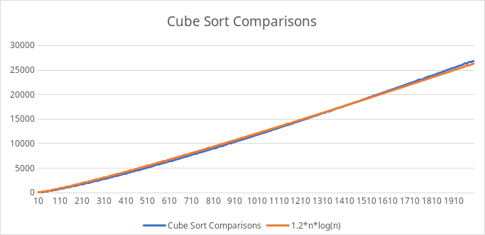
On the scales that I worked with, cube sort ends up with a time complexity of 1.2*nlog(n). I think this is mostly the case because we’re never adding all the items to a perfectly balanced cube so it ends up being inefficient at times.
Also, log(n) is a much more powerful function than sqrt(n) so including some square roots actually decreases its efficiency. Not only that, but log(n) is also more efficient than 4*log(n/4) so splitting it into multiple binary searches doesn’t help either.
The most efficient sorts tend to be slightly below the level of nlog(n) while Cube Sort lies slightly above that. The cube data structure also uses a lot of memory overhead to account for all the different axes so it’s not efficient memorywise either.
Inserts
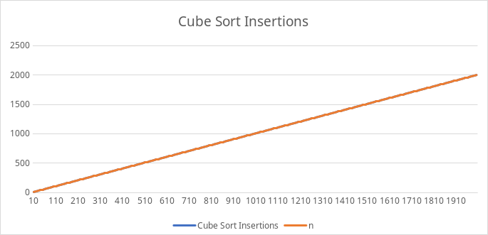
Insertions are much simpler. Since they’re only done to traverse the cube and insert into the array, it’s only a time complexity of n.
Distribution
This is how the comparisons and insertions are distributed for this sorting algorithm of size 100 for 1,000,000 sorts.
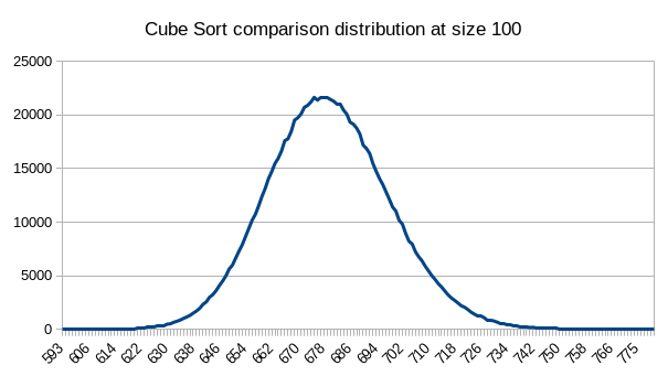
Mode: 677
Mean: 679
Std dev: 18
Max: 794
Min: 593
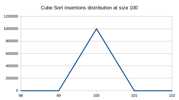
Mode: 100
Mean: 100
Std dev: 0
Max: 100
Min: 100
These distributions are fairly standard. Comparisons are distributed in a normal distribution around the mean and insertions are always equal to n.
Remember that these are done with a 4D binary search tesseract.
Cube sort C code
The code for this is a bit too long, so I’ll link to it here: